English
 Español
Basic Concepts
Understanding fundamental concepts is essential for developing efficient and sustainable solutions focused on irrigation. This first module brings together the main topics that will serve as the foundation for the content covered throughout the documentation.
Energy is not created or destroyed.
This fundamental principle:
- Encompasses all forms of kinetic, potential, thermal, radiant, electrical energy and its equality with mass;
- Is behind many of the equations used in Irrigation and Hydrology;
- Continuity;
- Work-Energy (Bernoulli);
- Water movement in soil (Van Genutchen);
- Crop water balance;
The principle was applied in structuring the Water Resources and Irrigation Projects records, allowing its application in validation and analysis of movements at various levels of the irrigation structure.
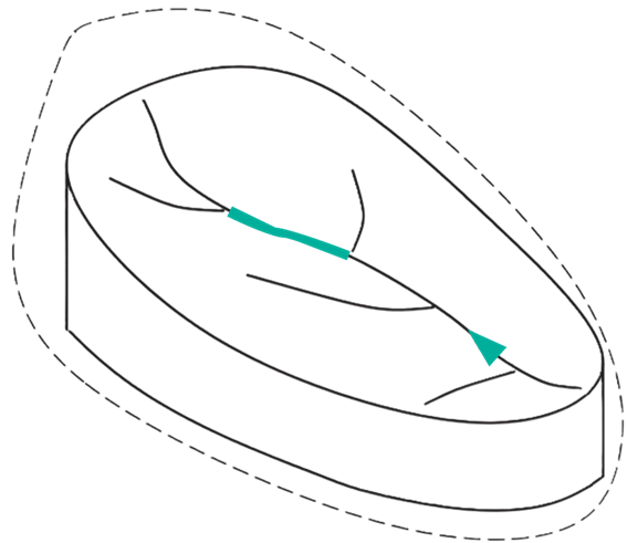
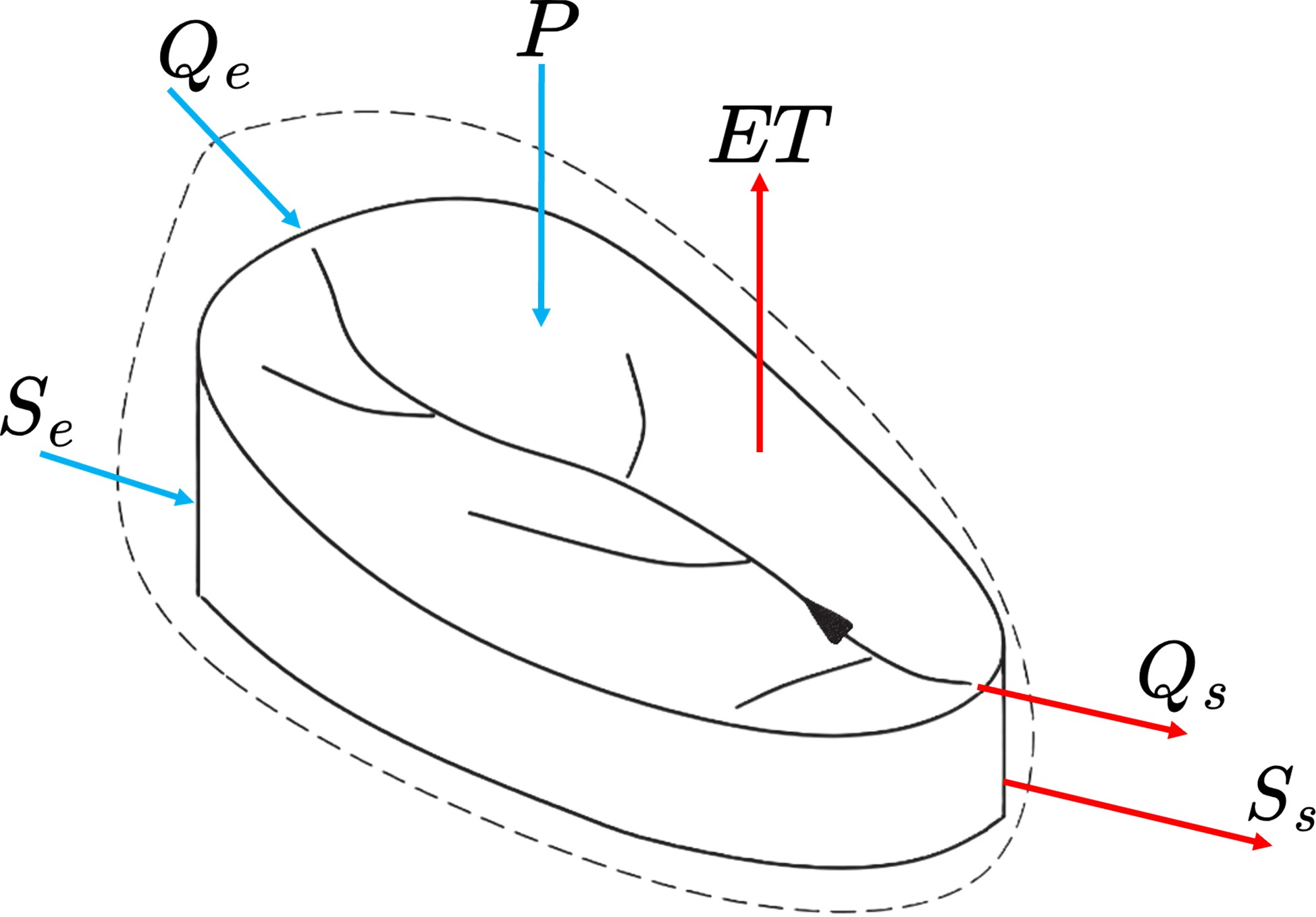
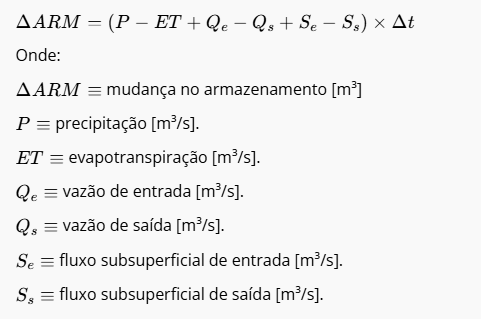
Closed region of finite size, where we can apply the principle of energy conservation and accounting to track water and energy inflows and outflows.
The change in energy in a control volume, during a time interval, must be equal to the amount of energy that entered minus the amount of energy that exited.
In the system, the following are considered control volumes:
- Watersheds
- Watercourses
- Water bodies
- Irrigation projects
- Conduits
- Command areas
- Agricultural sites
- Farms
- Blocks
- Plots
The figure below illustrates some of the variables involved in the flow of a title through a closed conduit.
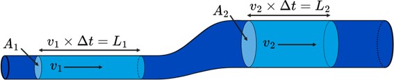
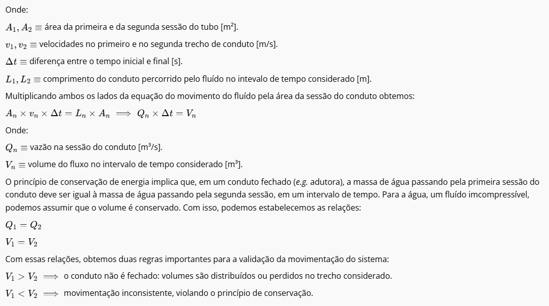
We can apply the continuity principle to account for control volumes, knowing the inflow and outflow.
The mass of water conserved in the control volume must be equal to the sum of the inflow and outflow, multiplied by the time interval considered, as described in the equation below:
These data extractions are not yet in the system, but can be easily implemented given its structure.
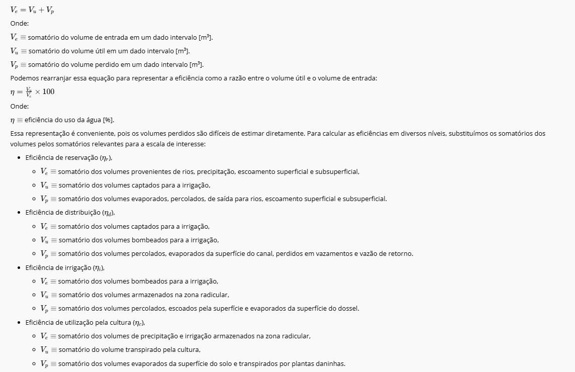
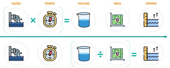
Combining the relationships presented previously, we can obtain water use efficiency at various scales. The input volume of a system is equal to the sum of the volume used and the volume lost:
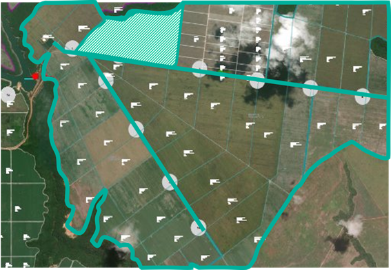
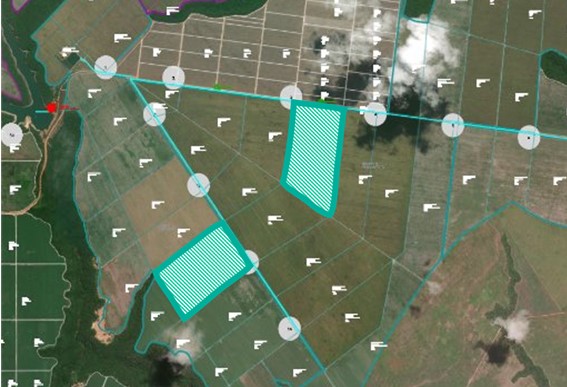
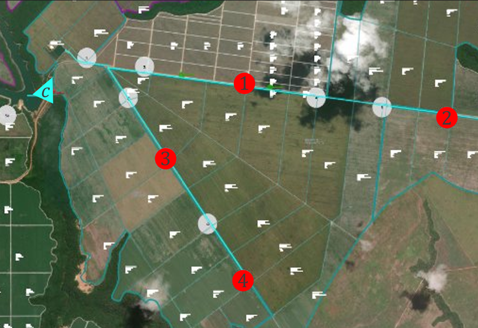
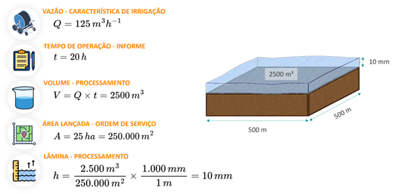
The figure below represents an irrigation project with the derivation (distribution via channel) of the volumes captured at point C to four water pumping points for irrigation, we will use this representation to demonstrate the calculation of distribution efficiency.
The volume of inflow in the control system is represented by the product of the average flow rate of the intake and its operating time:

We can expand the application of the conservation principle to describe the work - energy relationship in the constant flow of fluid in a pipe. Below we add variables representing this relationship to the diagram of a pipe section presented previously.
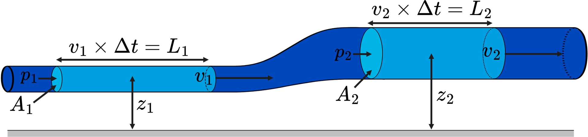
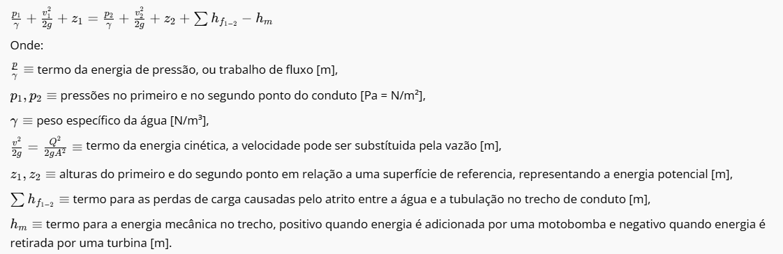
The Bernoulli equation mathematically describes these relationships and the conservation principle through the equality between two points of the conduit, the terms were arranged so that the resulting unit is the meter:
Using the same structure presented for water use efficiency, we can apply the Bernoulli equation to analyze the losses and gains of energy in irrigation projects. In this way, it is possible to determine the energy efficiency of irrigation projects at different scales and identify improvement points.
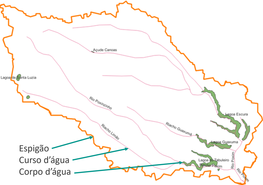
Water resources are grouped into watersheds:
- Delimited by a geographical feature, ridge, that makes precipitation flow to its axis;
- Considered as a control volume, as well as the bodies and watercourses that compose it;
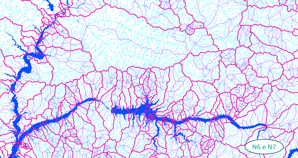
- Can be described at various levels, according to the Otto Pfafstetter ottocoding;
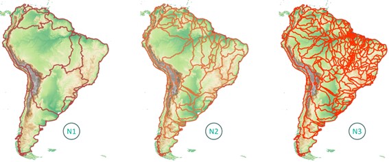
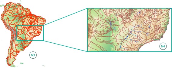
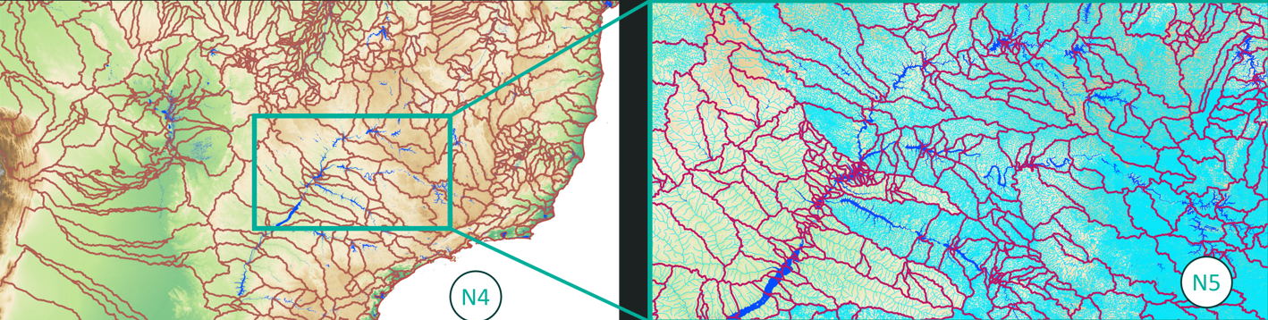
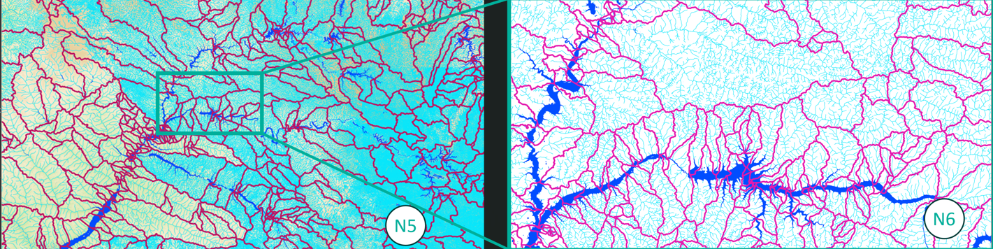
The Agência Nacional de Águas e Saneamento Básico (ANA) classified the hydrographic basins of our territory into seven levels: Otto Level 1, continental, to Otto Level 7, microregions. These levels are illustrated in the figures below.
The chosen Otto levels, as well as the hierarchical representation of water resources in the system, are choices of the managers and depend on the level of control expected to be obtained in the system. ANA maintains a database with all the water resources of our territory on the Sistema Nacional de Informações sobre Recursos Hídricos portal, a valuable reference for irrigation professionals.
The irrigation project, normally, groups the infrastructure implemented from a single hydraulic design and supplied by freshwater from a single point (or section) of interference of a water use grant.
- Set of structures and hydraulic machines, irrigation infrastructure;
- Capturing fresh or wastewater;
- Distributing this water through:
- Adduction, in closed (adduction pipelines) and pressurized conduits;
- Derivation, in open conduits (canals), by gravity;
- Irrigating agricultural fields;
- Transferring water to reservoir structures.
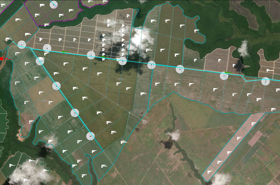
To characterize the irrigation project, we use definitions from the literature to create nodes that represent its structure.
- Irrigation project - groups the water supply infrastructure.
- Pumping - represents the location and/or infrastructure used in the capture and pumping of water for irrigation, as well as the associations between the motor pumps.
- Conduit - represents the open conduits, canals, and closed conduits, adduction pipelines, used in the derivation and distribution of water.
- Water resources - represents the water resources interspersed in the project structure, such as aeration tanks and targets for transfer.
- Command area - set of effectively irrigated areas of the project, served by a single type of irrigation system.
- Sector - managerial and/or hydraulic division of the command area.
- Chemigation - represents the infrastructure used for the injection of agricultural inputs into the irrigation water.
Pumping nodes have some special characteristics. Connections between pumping nodes and motor pump allocations at the node can be used to represent series and parallel associations.
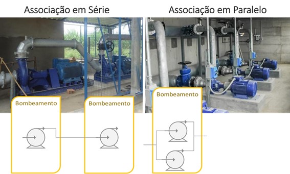
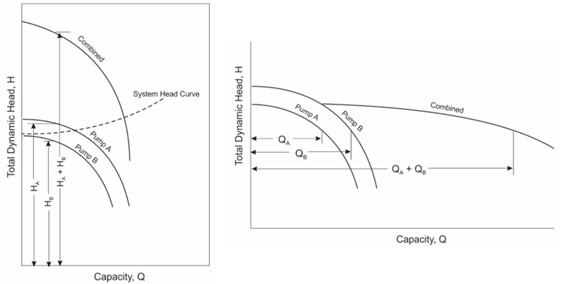
These associations have distinct effects. The series association results in the sum of the dynamic pressures of the motor pumps, and the parallel association in the sum of the equipment flow rates. The effects of the series association are not yet covered by the system, requiring the hydraulic description of the conduits. The parallel associations have an effect on the accounting of the volumes produced by the pumping nodes, according to the graph on the right (figure below).
The correct dimensionality of the entities used in irrigation is important to maintain the significance of what we want to represent and ensures the coherence of the calculations performed in irrigation management, therefore, we must pay attention to the compatibility between entities, dimensions and units of measurement used in their representation. We can arrive at the main quantities of interest for irrigation through dimensional analysis.
| Dimension | Quantity | Notations |
|---|---|---|
 |  | * Depth - L in dimensional analysis notation * Expressed in millimeters (mm) * 1 mm = 0.001 m ≡ 1 l/m2 |
 |  | * Irrigated Area - L² in dimensional analysis notation * Expressed in hectares (ha) * 1 ha = 10,000 m² |
 |  | * Irrigated Volume - L³ in dimensional analysis notation * Expressed in cubic meters (m³) * 1 m³ = 1000 l |
 |  | * Operating Time - T in dimensional analysis notation * Expressed in hours (h) * 1 h = 60 min = 3600 s |
 |  | * Flow Rate - L3/ T in dimensional analysis notation * Expressed in cubic meters per hour (m3/h) * 1 m³/h = 1,000 l/h ≃ 0.278 l/s |
The calculation of depth and its significance depends on the area used in the calculation. Below are the nomenclatures of the areas used in the system and variables obtained from them:
- Topographic area: From the agricultural site registration and used in the calculation of irrigation depth.
- Planned area: Informed at the opening of the service order and used in the calculation of planned depth, adherence, and completeness.
- Irrigated area: A function of the irrigation system and its operation data, used in the calculation of report depth and overlap.
- Posted area: Sum of the areas posted in the service order, representing the effectively irrigated area, used in the calculation of performed depth, adherence, completeness, and number of depths.
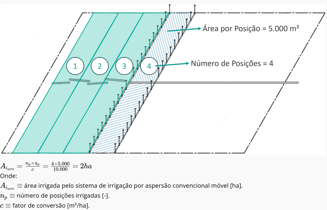
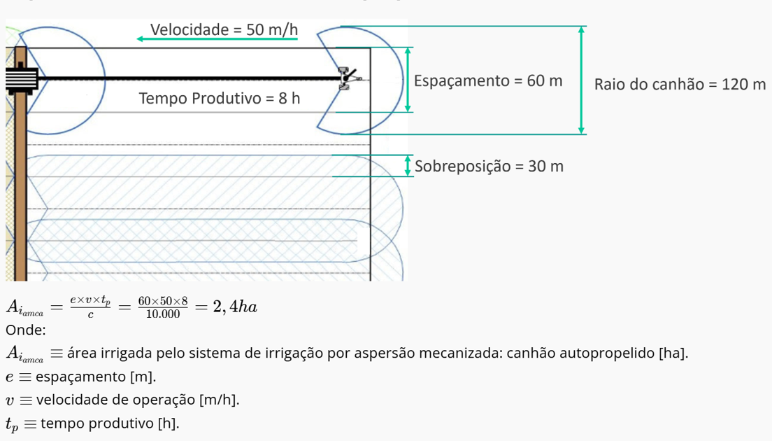
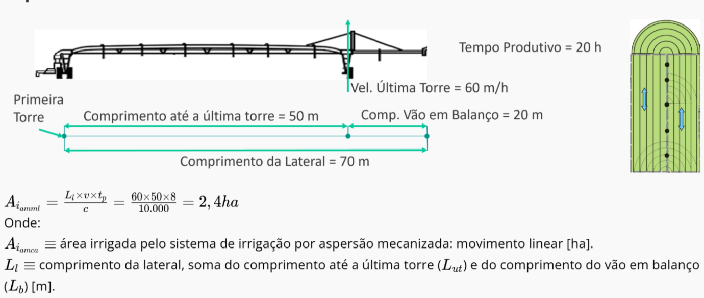
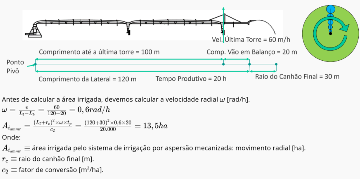
- Irrigated Area: Calculated based on the irrigation system and equipment operation data. For fixed irrigation systems, the irrigated area equals the sum of the areas of the sectors that make up the command area, registered in the irrigation project tree. For other systems, the calculations are shown below:
The classification of irrigation equipment in the system is essential for its characterization, association with the project structure, and processing of operation data. Below, we have a dichotomous key for the classification of irrigation equipment:
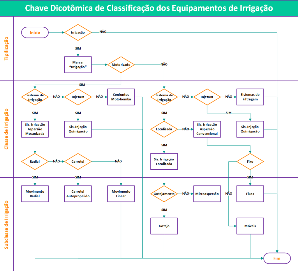
The equipment taxonomy controls the availability and dimensionality of the irrigation characteristics available for describing model versions.
| Variable | Unit | Unit Type | Pump Sets | Conv. Fixed Sprink. | Conv. Mobile Sprink. | Mech. Reel Sprink. | Mech. Linear Sprink. | Mech. Radial Sprink. | Drip Irrig. | Micro-sprink. Irrig. | Fertigation | Filtering |
|---|---|---|---|---|---|---|---|---|---|---|---|---|
| Design Flow Rate | L³/T | Flow | 1 | 1 | 1 | 1 | 1 | 1 | 1 | 1 | 1 | 0 |
| Design Pressure | M/LT² | Pressure | 1 | 1 | 1 | 1 | 1 | 1 | 1 | 1 | 1 | 0 |
| Design Rotation | 1/T | Frequency | 1 | 0 | 0 | 0 | 0 | 0 | 0 | 0 | 1 | 0 |
| Pump Efficiency | % | Dimensionless | 1 | 0 | 0 | 0 | 0 | 0 | 0 | 0 | 1 | 0 |
| Rotor Diameter | L | Length | 1 | 0 | 0 | 0 | 0 | 0 | 0 | 0 | 1 | 0 |
| Application Efficiency | % | Dimensionless | 0 | 1 | 1 | 1 | 1 | 1 | 1 | 1 | 0 | 0 |
| Spacing on Line | L | Length | 0 | 1 | 1 | 0 | 1 | 0 | 1 | 1 | 0 | 0 |
| Spacing between Rows | L | Length | 0 | 1 | 1 | 1 | 0 | 0 | 1 | 1 | 0 | 0 |
| Maximum Flow Rate | L³/T | Flow | 1 | 1 | 1 | 1 | 1 | 1 | 1 | 1 | 1 | 0 |
| Minimum Flow Rate | L³/T | Flow | 1 | 1 | 1 | 1 | 1 | 1 | 1 | 1 | 1 | 0 |
| Maximum Rotation | 1/T | Frequency | 1 | 0 | 0 | 0 | 0 | 0 | 0 | 0 | 1 | 0 |
| Minimum Rotation | 1/T | Frequency | 1 | 0 | 0 | 0 | 0 | 0 | 0 | 0 | 1 | 0 |
| Lateral Length | L | Length | 0 | 0 | 1 | 1 | 1 | 1 | 0 | 0 | 0 | 0 |
| Non-Irrigated Length | L | Length | 0 | 0 | 0 | 0 | 0 | 1 | 0 | 0 | 0 | 0 |
| Number of Emitters | - | Dimensionless | 0 | 1 | 1 | 1 | 1 | 1 | 1 | 1 | 0 | 0 |
| Advance Time | T | Time | 0 | 1 | 1 | 1 | 1 | 1 | 1 | 1 | 0 | 0 |
| Emitter Nozzle Diameter | L | Length | 0 | 1 | 1 | 1 | 1 | 1 | 0 | 0 | 0 | 0 |
| Emitter Discharge Coefficient | - | Dimensionless | 0 | 1 | 1 | 1 | 1 | 1 | 0 | 0 | 0 | 0 |
| Average Pressure on Lateral | M/LT² | Pressure | 0 | 1 | 1 | 1 | 1 | 1 | 1 | 1 | 0 | 0 |
| Average Emitter Flow Rate | L³/T | Flow | 0 | 1 | 1 | 1 | 1 | 1 | 1 | 1 | 0 | 0 |
| Overhang Span Length | L | Length | 0 | 0 | 0 | 0 | 1 | 1 | 0 | 0 | 0 | 0 |
| End Gun Radius | L | Length | 0 | 0 | 0 | 0 | 1 | 1 | 0 | 0 | 0 | 0 |
| Number of Sets | - | Dimensionless | 0 | 0 | 1 | 0 | 0 | 0 | 0 | 0 | 0 | 0 |
| Standard Travel Speed | L/T | Speed | 0 | 0 | 0 | 1 | 1 | 1 | 0 | 0 | 0 | 0 |
| Wetted Radius | L | Length | 0 | 0 | 0 | 0 | 0 | 0 | 0 | 1 | 0 | 0 |
| Tank Volume | L³ | Volume | 0 | 0 | 0 | 0 | 0 | 0 | 0 | 0 | 1 | 0 |
| Inlet Pressure | M/LT² | Pressure | 0 | 0 | 0 | 0 | 0 | 0 | 0 | 0 | 0 | 1 |
| Outlet Pressure | M/LT² | Pressure | 0 | 0 | 0 | 0 | 0 | 0 | 0 | 0 | 0 | 1 |
| Minimum Outlet Pressure | M/LT² | Pressure | 0 | 0 | 0 | 0 | 0 | 0 | 0 | 0 | 0 | 1 |
 English
 Español